Precise Locating on Complex Geometries

Sometimes you might want to put something on a specific spot on a complex shape. Like a hole for passing wires, or an instrument for measuring load, strain, acceleration, or some other phenomenon.

The Problem

How do I easily put a mark on some real life complex surface and know its CAD coordinates and vice versa?

I have seen this problem solved using plumb bobs, spirit levels, a level floor, and a lot of time measuring. This problem can also be solved with specially marked places on the real life object that have known coordinates, then measuring arc lengths along the surface towards the spot you want. These solutions do not provide accounting of their quality, and do not generalize well to many locations. For instance, if you were to be asked “How close is that Preston Tube port on the aircraft to the spot you marked in CAD?” you would have to say something like “I hope its pretty close.”

I propose a method that will allow easier, more accurate locating on a complex geometry, with quantifiable error.

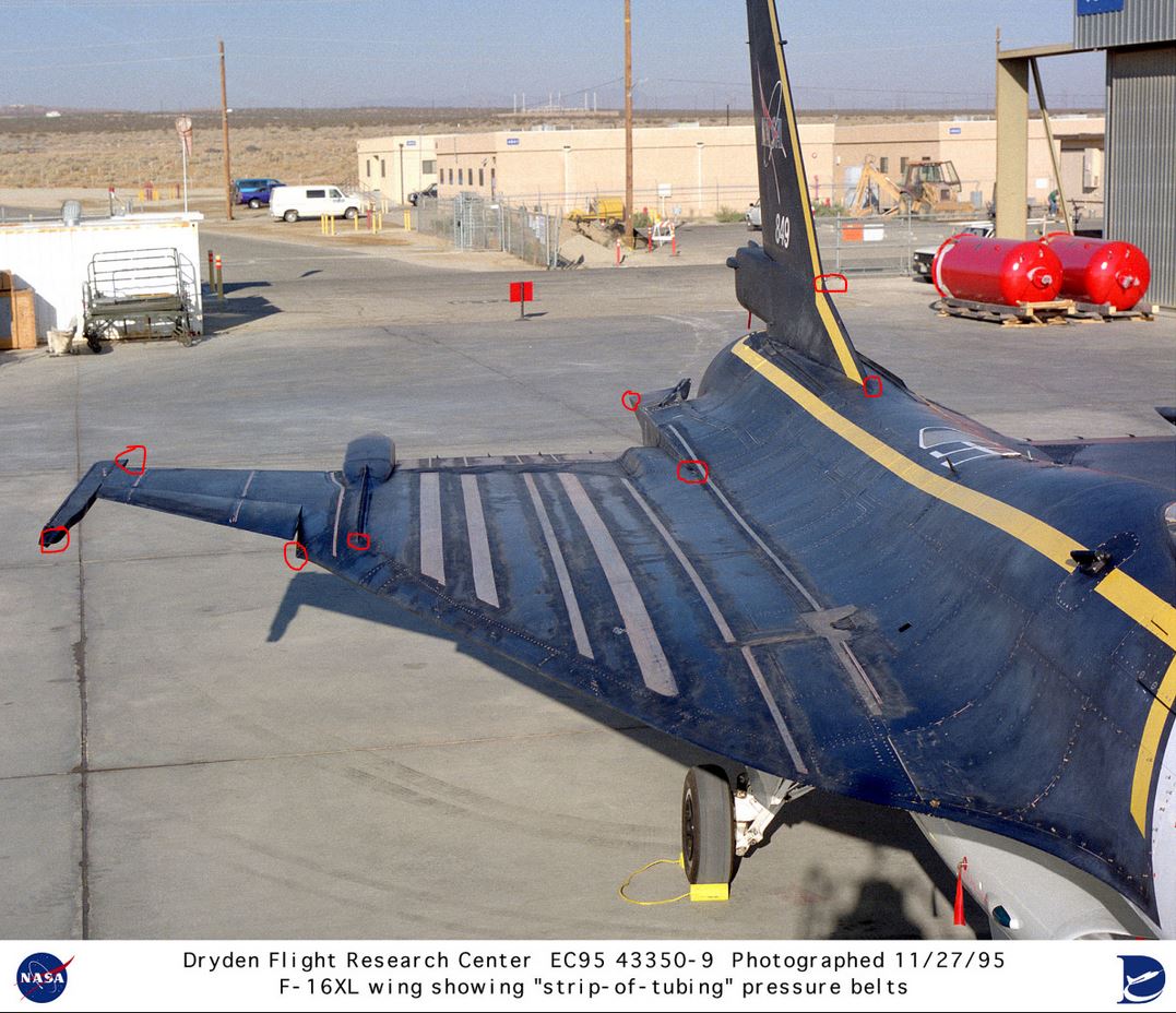
If you cant visualize this problem, let me give a specific example. This is an F-16XL flown by NASA:

NASA used this F-16XL as a test-bed for research projects. They measured local skin friction with these small “Preston Tubes” shown in the photo below.

Nowadays, if you were in charge of choosing where to put these tubes, you would probably use a CAD program. Lets imagine NASA has a model for local skin friction over the wing, and they’re trying to validate it. An engineer chooses locations to place the tubes via CAD and now they want to mark said locations on the airplane.

What Lurks in the Details

You (I am now calling this imaginary engineer you) march over the airplane knowing where your tubes should be placed. You might have their exact locations called out in your Cartesian CAD coordinates like so:

Preston Tube	X	Y	Z
pt_0	463.62	755.32	1120.34
pt_1	481.05	761.23	1145.88
…	…	…	…
pt_n	n_x	n_y	n_z

If you’re unlucky, you have to find where these X,Y,Z locations are yourself. Now you’re in the hangar looking up at this thing (pictured below) thinking “Where is X 463.62, Y 755.32, and Z 1120.34?”

The dreadful moment has come, when you realize it is hard to go from CAD coordinates to a real life X marks the spot. (An additional complication not covered here is that airplanes are not completely rigid, they bend and flex with different fuel quantities, cargo loading, tire pressures, gear loading, wing loading, etc.) I assume in this article that the CAD geometry can be replicated in real life. This assumption becomes increasingly valid the more rigid the body, and the more localized your area of interest.

The Solution – In Kabsch we Trust

The solution is to measure a series of known points from a fixed location relative to the complex object, and then find the linear transformation (a translation and a rotation) that minimizes the root sum of the squared distances between each point in one coordinate system and its pair in the transformed system. This is not a novel idea, the algorithm to compute such a transformation is called the Kabsch Algorithm. The question is now, how do I make use of the algorithm.

A Translation, and Rotation that Minimizes RMSE

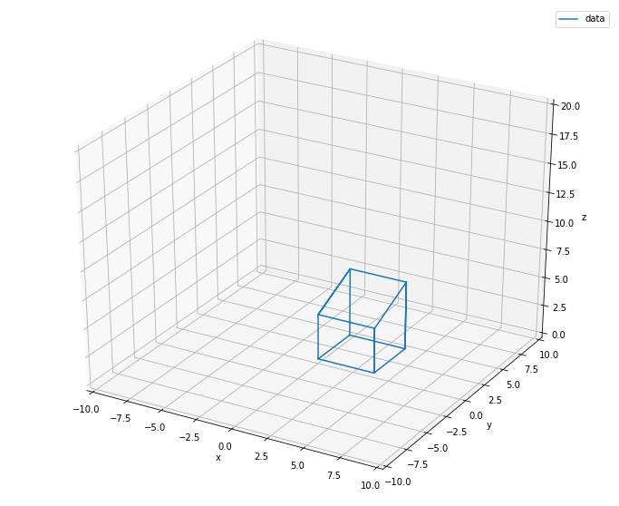
I’ll show an example so that its clearer to me and my tremendous reader-base. Imagine your CAD object looks like so:

And imagine that in real life, your object hangs from the ceiling like this (in orange):

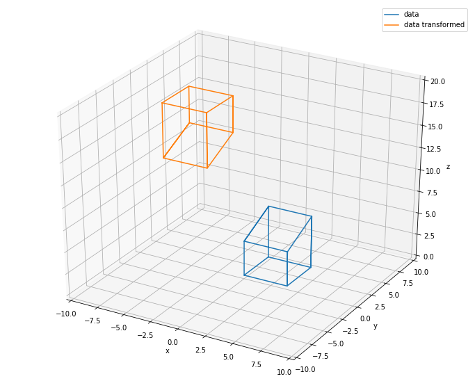
You can probably visualize flipping the orange object (rotating it about some axis) and then moving it until it overlays the original CAD object like so:

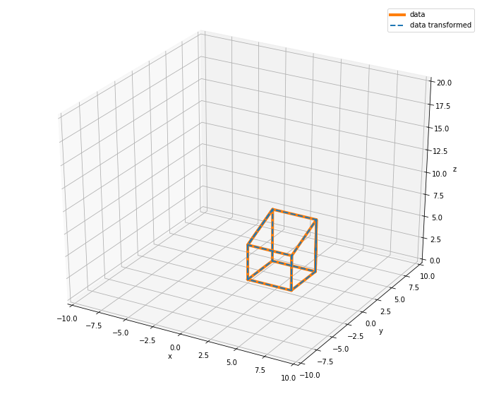
This is the gist of what the algorithm accomplishes and the method I propose. “But what about minimizing the root sum of squared distances?” I can hear the audience shouting. In the above case, the data was transformed exactly on top of its CAD geometry, and the distance between each pair of measured points is 0, therefore the RMSE (root mean squared error) is 0. The formulation for calculating RMSE is below.

$$RMSE = \sqrt{\frac{1}{n}\sum_{i=1}^{n}(y_i-x_i)^2}$$

Where \(y_i\) is the coordinate measured in CAD and \(x_i\) is the coordinate measured in real life. \(n\) is the total number of points measured. When there is some error in measuring the location of points (like in real life), the overlaying of one object on the other will not be exact BUT that error is quantifiable in the form of RMSE.

The Solution in Real Life

Going back to the aircraft example, you’re armed with CAD coordinates where you want your Preston Tube ports to be located. You are looking at the airplane with the desire to mark those locations out on the physical surface.

To implement the kabsch algorithm, you will need some additional equipment, namely a way to generate points in some new coordinate system. This can be done with a laser distance measurement device and a precise way to measure 2 angles (the equivalent of measuring \(r\), \(\theta\), and \(\phi\)) in spherical coordinates which are easily transformed into Cartesian coordinates. Or a more advanced device like the Leica Disto S910 which can output Cartesian coordinates directly.

You will also need to know the CAD coordinates of some easily found points on the complex surface you would like to mark locations on. In the case of the F-16XL, some obvious candidates are marked out in red circles below:

These “known” points have known CAD coordinates AND are easily recognizable on the aircraft such that they may be measured precisely from a fixed location. When I write “measured precisely from a fixed location” I mean something like this:

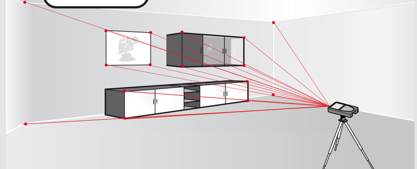
By measuring the known CAD points that are easily identifiable on the aircraft, you can generate a table like this:

Point	Measured X	Measured Y	Measured Z	CAD X	CAD Y	CAD Z
Trailing Wing Tip	526.51	251.12	690.15	…	…	…
Vertical Stab Meets Fuse	693.73	293.33	195.56	…	…	…
Fuse Body Joint	…	…	…	…	…	…
Stall Fence Leading Joint	…	…	…	…	…	…

Now using the Kabsch algorithm you can find the transformation that will allow you to make any measurement in real life, and transform it into CAD coordinates or vice versa. I’ll show it visually and in words below:

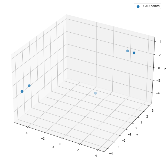
These are the 5 points you found in their CAD coordinates that are easily located on your complex geometry:

Now the 5 points in orange below are what you measured in real life (like in the cabinets picture):

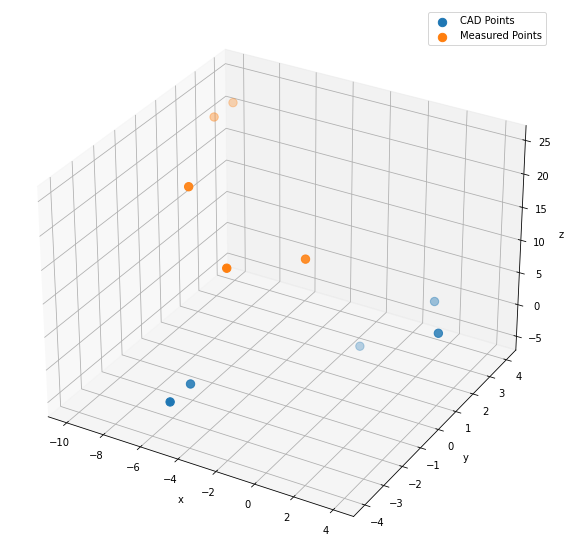
Now, there exists some translation and rotation (a linear transformation) that minimizes the distance between the points. and that transformation can be applied to any newly measured points to give its CAD coordinates.

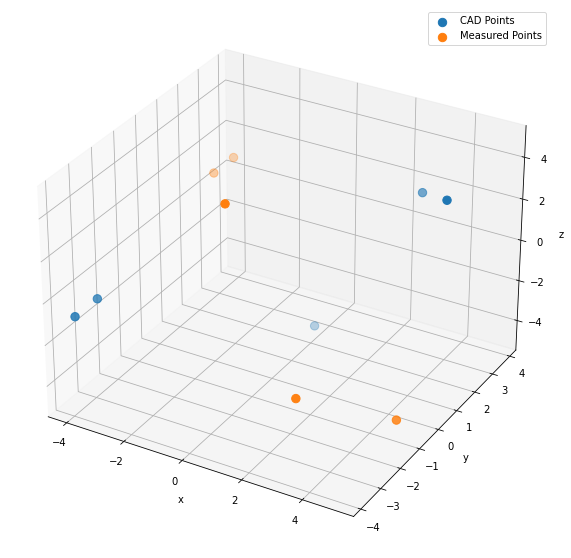
First, subtract the centroid of each point cloud from all points in that cloud. This centers both the measured and CAD points around 0. Visually, they will look like so:

Now, apply the Kabsch algorithm, comprised of computing the covariance matrix of the two point clouds. The singular value decomposition of the covariance matrix, correcting for a right-hand coordinate system if necessary. Finally, using the \(V\) and \(U\) matrices from the SVD to compute the optimal rotation matrix \(R\). The matrix math involved is clarified on the Kabsch algorithm Wikipedia page. An implementation in python exists here. Using that python implementation on the two point clouds above:

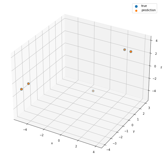
Armed with the rotation matrix \(R\), the centroids of the measured and CAD coordinates, any new measured point can be converted into the CAD coordinates.

$$CAD\ Coordinates = (P-B)R+A$$

Where \(P\) is a new measured point \([P_x,P_y,P_z]\)to be converted to CAD coordinates. \(B\) is the centroid of the known measured coordinates. \(R\) is the rotation matrix. \(A\) is the centroid of the known CAD coordinates.

In English, the above formula states that the CAD Coordinates are equal to the known measured coordinates, minus their centroid, times the rotation matrix found via Kabsch, plus the centroid of the known CAD coordinates.

Now, any measurement done from your fixed location via your laser or alternative measurement device can be easily converted to CAD coordinates.

Doing This Yourself

Here are the steps to making this process work for you on a complex geometry:

1. Start with a CAD model of the geometry.
2. Locate the points in CAD you want to mark on the object and note their coordinates.
3. Locate points in CAD that are easily identifiable on the actual object and note their coordinates I’ll refer to these as the known points.
4. From a fixed location, measure the known points in real life and note their measured coordinates. (now you have 3 sets of coordinates).
5. Pass the measured and CAD coordinates of known points as matrices into the python implementation of the Kabsch algorithm I linked above.
6. This algorithm returns the predicted location in CAD coordinates of the measured points (plot these in CAD to see how close they are to the actual CAD locations). The algorithm also returns a rotation matrix and a translation vector.
7. Measure approximately where you want to mark the actual object, and convert the measured coordinates to CAD.
8. Iterate on this approximation getting closer to the CAD location you want to mark until you are satisfied with the accuracy of your location.
9. Mark the object.

Here are some tips to make the best of this solution:

• Measure at least 4 known points with variation in all 3 CAD coordinate axes, ideally near the locations you want to mark.
• If your object is outside and you’re using a laser, consider measuring at night.
• Note coordinates in a file or programatically so that you may easily work with the data.
• Don’t move your measurement device during the process or you will need to start over.
• Quantify the error of your transformation with the RMSE of the transformed known points.