Introduction
In my last post I developed a flight dynamics model (FDM) using data from a fixed wing RC plane containing the Pixhawk1 running Ardupilot firmware. I suggested that I should look into the following:
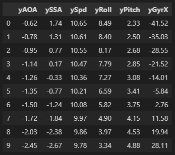
Visualize a learned model’s relationship between control inputs and state variables. For instance, does the model learn what we might expect about aileron inputs and roll?
In this post I will peek into the black box model developed and see what we can find.
What Sayeth the Neural Network
There is a handy book on Interpretable Machine Learning by Christoph Molnar that provides 2 methods that will be useful for trying to understand if the FDM matches expectations. The first is the Individual Conditional Expectation (ICE) plot, and the second is the Partial Dependence Plot (PDP). He explains them well in the book, but I will cover them more haphazardly for this particular application.
Individual Conditional Expectation (ICE) Plot
The Individual Conditional Expectation plot shows how a model response changes as you vary one of the model’s predictors. Here is a subset of columns from a single sample of flight data:
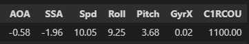
At some discrete time \(t\), the aircraft had the above measurements – I’ll refer to the entire set of measurements at any given time as the “state” of the aircraft. Everything shown is measured in degrees except for:
- Spd (horizontal ground speed) is measured in meters per second
- GyrX which is measured in radians per second and indicates a roll rate about the X axis (see below).
- C1RCOU which stands for Channel 1 Remote Control Output – it is a measure of the pulse width sent to the aileron servos (connected to output channel 1). Generally 1000 indicates max deflection one way and 2000 indicates max deflection the other way.
I can pass the state of the aircraft at time \(t\) into the trained model to predict the state of the aircraft at time \(t+\Delta t\). (In this case \(\Delta t\) is 0.1 seconds) I can also change the current state of the aircraft and see how the future state prediction changes. This is what the ICE plot shows.
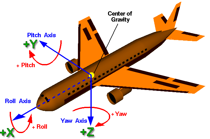
Imagine that I take C1RCOU (aileron position) and adjust it through its full deflection – making a prediction about the next “state” of the airplane at each incremental adjustment. The input looks like this:
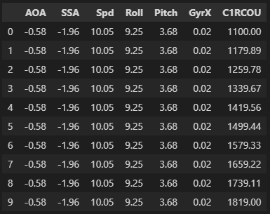
Notice how everything is kept constant except for C1RCOU, which is adjusted through its range observed in the training data. Predicting on each sample, the prediction output looks like this:
I prepended the output columns with a y to clarify they are outputs from the model. Notice that the model adjusts all of the outputs as a function of aileron deflection (C1RCOU) – but some things – Roll Rate (yGyrX) change more than ground speed (ySpd) which makes sense! Lets look at the ICE plot showing how roll rate is a function of aileron deflection for this sample:
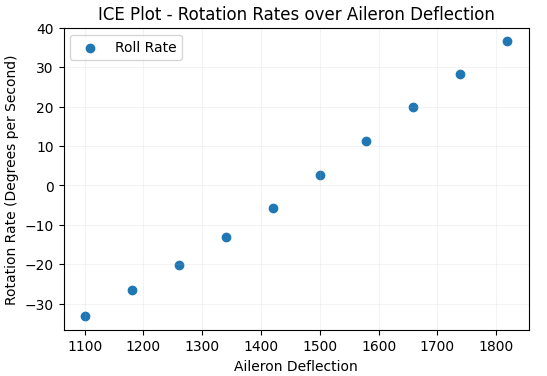
For this sample, roll rate is monotonically related to aileron deflection which is intuitive. Increased aileron deflection in either direction should generally correspond to an increase in roll rate in either direction. It’s also possible to look at how aileron deflection affects side slip and pitch rates:
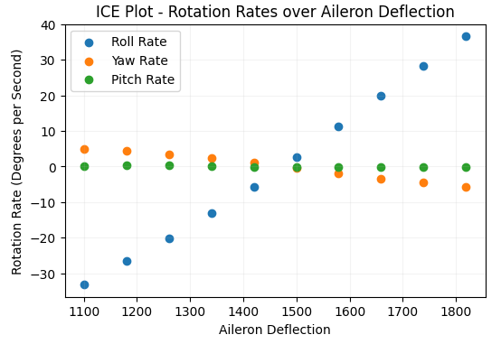
Notice that the magnitude of the effect on yaw and pitch rates is much lower than the effect on roll. This makes it seem like the model developed a sensible relationship between aileron deflection and rotation rates. Correspondingly, I expect the model to capture a monotonic relationship between elevator deflection and pitch rate, with small effects on roll and yaw rates.
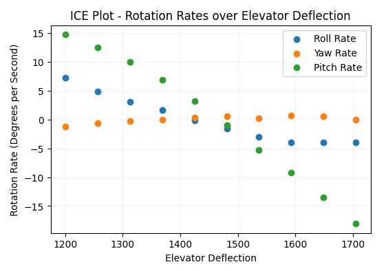
The model does show a monotonic relationship between elevator deflection and pitch rate – but it also shows interesting change in yaw and roll rates as the elevator is deflected. Still – it is good to see that the dominant effect of elevator input is a rotation rate in pitch.
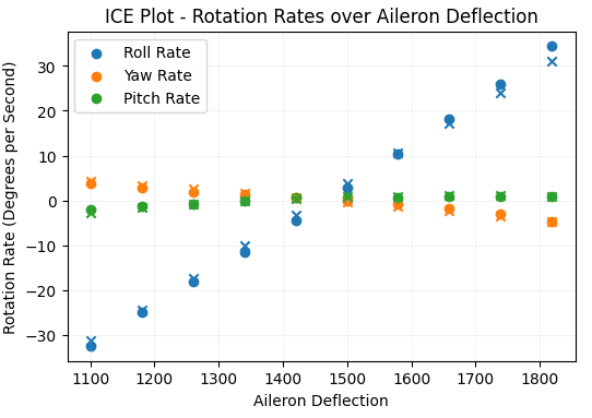
This is an extremely limited perspective, as this only shows one sample of test data. One issue could be that the aircraft is stalled in the sample I chose, so the control surfaces should not be very effective, and the model may have picked up on that. This kind of complex situation is unlikely. The model does not have much training data and is very unlikely to have “understood” interaction between airspeed and control authority near stall speed – still this is something that can be explored using ICE plots. The plot below shows the relationship between aileron deflection and rotation rates in 3 axes at 2 different speeds. X’s represent a flight speed of 24mph and dots represent a flight speed of 13mph. Notice that the roll rates are not greater at higher airspeed as one would expect with the increased control authority at higher airspeed.
ICE plots are useful for detecting interaction between variables that feed into the model. As more samples are used and shown on the same plot, more sophisticated relationships can be discovered. For developing a general understanding of the model behavior (without considering interaction) I’ll look at the partial dependence plot.
Partial Dependence Plot (PDP)
The PDP shows the average relationship between a model’s output and its inputs. It is similar to the ICE plot – but instead of plotting single samples, the PDP averages over many samples. This comes with the clear limitation that interaction is not detectable with a one dimensional PDP. I’ll show some PDPs of the same variables explored above in ICE plots. If I average the many ICE lines I get from sampling from the test data and varying aileron position, I get this:
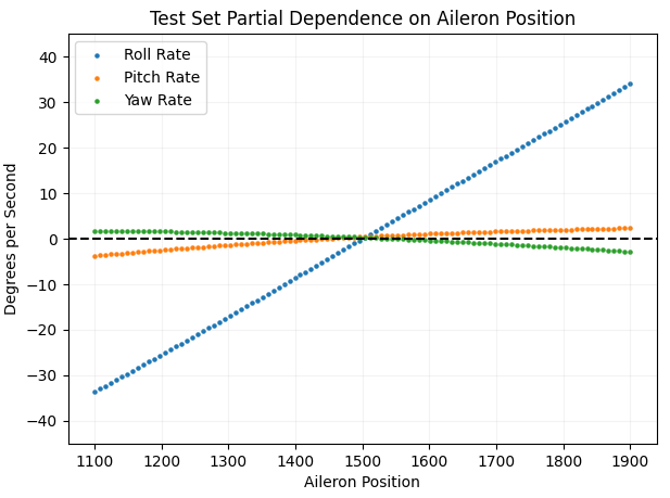
On average, changes in aileron position result in changes in roll, but also in a small amount of opposite yaw, which may be due to adverse yaw or simply error in the model. Now for the average effect of moving the elevator:
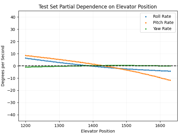
The result of changes in elevator position cause, on average, changes in pitch and roll rate, with no effect on yaw. Now for rudder position:
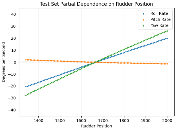
Interestingly, rudder has a very large effect on roll rate in addition to the effect on yaw rate. This airplane is sometimes flown with no ailerons – which makes sense given the relationship between rudder and roll rate shown by this flight dynamics model PDP. How about throttle:
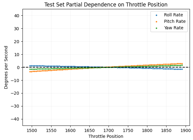
On average, changes in throttle position have a very limited effect on rotation rates… The thrust line of this aircraft is almost directly in line with the longitudinal axis, which is a desirable trait for limiting the effect of thrust on rotation rates. Something not achieved by this airplane:
Because the model predicts more than rotational rates – I can plot to check for other expected relationships, like throttle and accelerations.
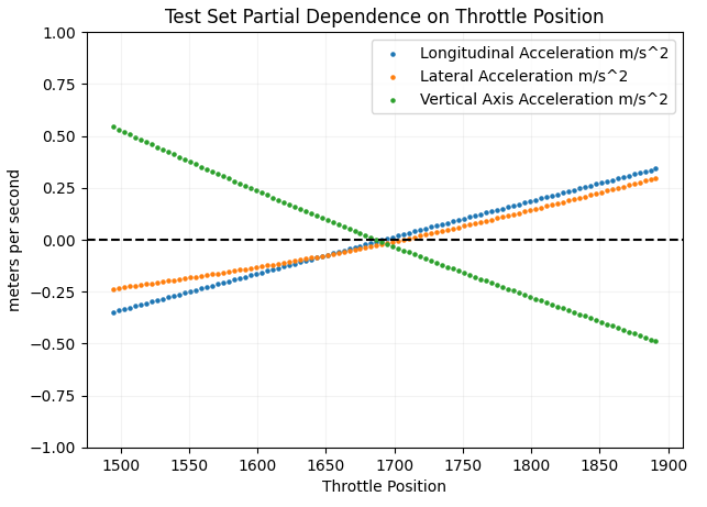
See above how throttle increases relate to an increase in longitudinal acceleration (makes sense), but interestingly it is even more strongly related to a decrease in z-axis (vertical) acceleration. I am actually not sure how to interpret this. Let me know if you have any thoughts.
To What the Neural Net Sayeth, Are we Listening?
This data-driven flight dynamics model is suspicious in a few ways shown by the ICE and PDP plots. I wouldn’t trust a control algorithm built using this FDM in simulation. How can we fix a rough data-driven FDM? I suspect more data is the easy (and mostly correct) answer. Without baking in any physics, or assumptions – there is a lot for the model to learn before it is useful in projecting aircraft behavior in response to control inputs. I suspect this dataset does not contain enough variation in the many dimensions used by the model. I wonder if a dimensionality reduction technique like PCA on the inputs to the model would help to speed up training, utilize a smaller network (faster prediction time), and require less data, without taking on a substantive reduction in model performance. Still to do from the last post:
- Get more flight data at a wide variety of conditions (flying aerobatics, inverted, stalls, etc.)
- Build a model that can run fast enough on hardware that can fit in the rats nest.