Introduction and Example
I have recently run into a feature engineering problem with regression analysis I have been doing at work. The issue is that not all independent variables that may be good predictors for a dependent variable are additive. Some might need to be multiplied together with some constant, or manipulated together before being included into the regression equation.
My attempt at a definition:
Interaction terms are terms in regression equations to represent non-additive interaction between variables.
A more thorough look at interaction can be found on the wikipedia page: https://en.wikipedia.org/wiki/Interaction_(statistics)
To visualize the importance of variable interaction, I have come up with the following example: A duct with one inlet, two outlets, and a valve controlling the flow to the outlets is instrumented and I will try to define the relationship between one of the outlets flow rate (our dependent variable) and two other measurements (input flow rate and valve position).

Bold items on the above system diagram are the features in the data set. The valve position controls the proportion of inflow that flows through the outflow. This system exists in some real life engineering applications such as waste-gates for turbochargers on internal combustion engines. https://en.wikipedia.org/wiki/Wastegate
I have created a sample time series data set for each of the three measurements:
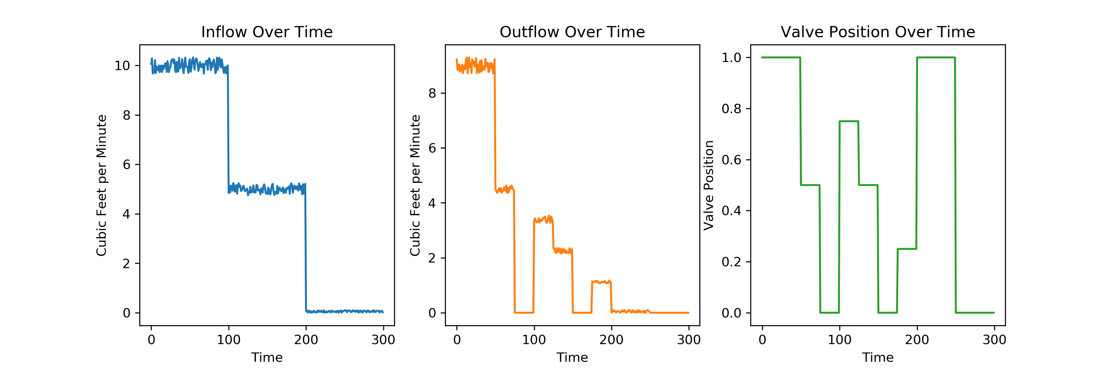
You can see clearly in the above plots, that the inflow starts at about 10 CFM, drops to 5, and then to 0. The outflow starts around 9, drops to half that at time 50, etc. The valve position varies between fully one way at value 1, and fully the other at value 0, with partial states between.
An excerpt from the dataset:
| Inflow | Outflow | ValvePos |
| 10.33 | 8.91 | 1 |
| 9.89 | 8.72 | 1 |
| 9.79 | 9.24 | 1 |
| 9.92 | 8.91 | 1 |
| 10.25 | 0 | 0 |
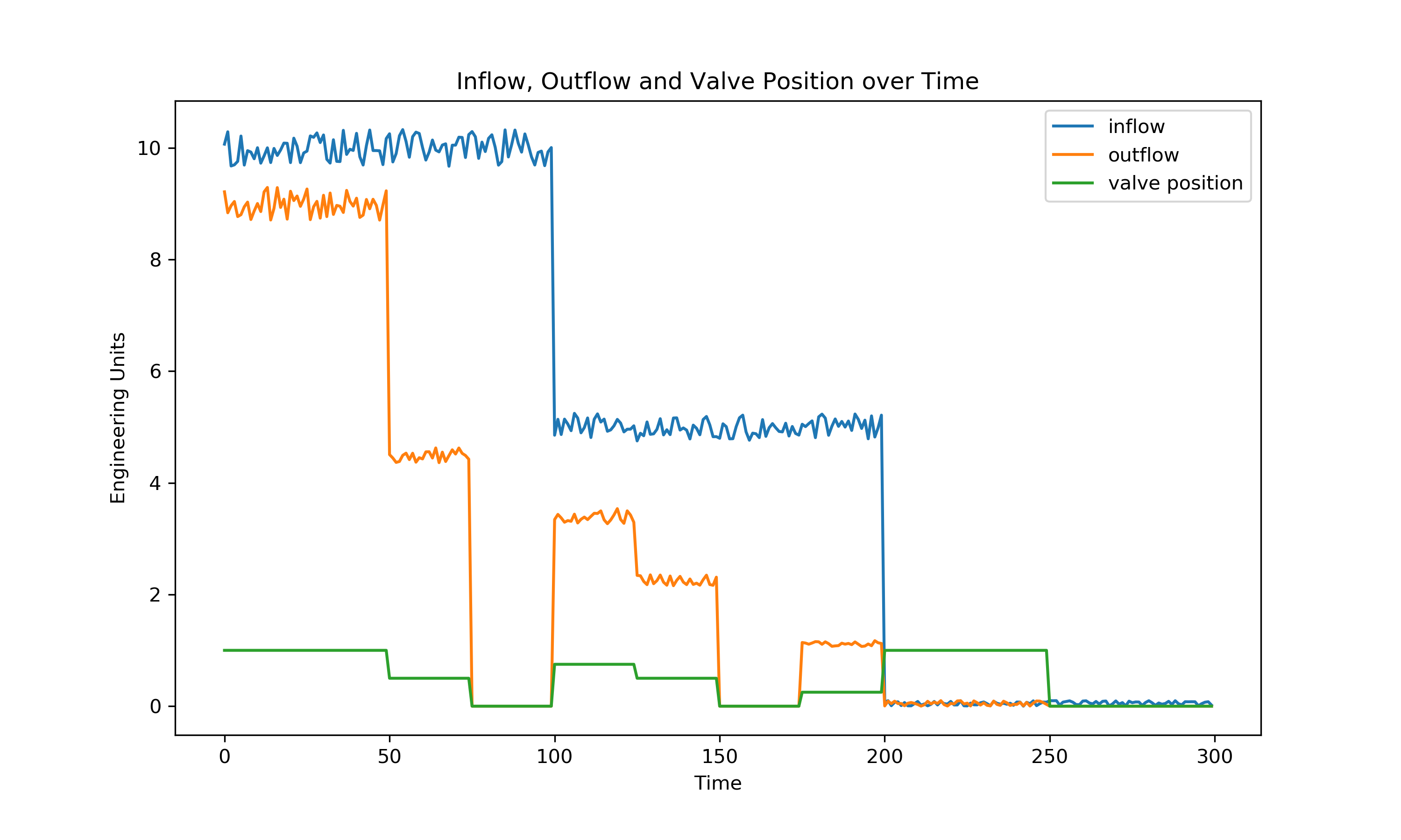
All together:
Simple Regression Model
I will build a baseline linear regression model using the python scikit-learn package to evaluate how well the model fits to the data with no interaction terms:
of_model = lr.fit(df.drop('outflow', axis=1), df['outflow'])

result = of_model.predict(df.drop('outflow', axis=1))
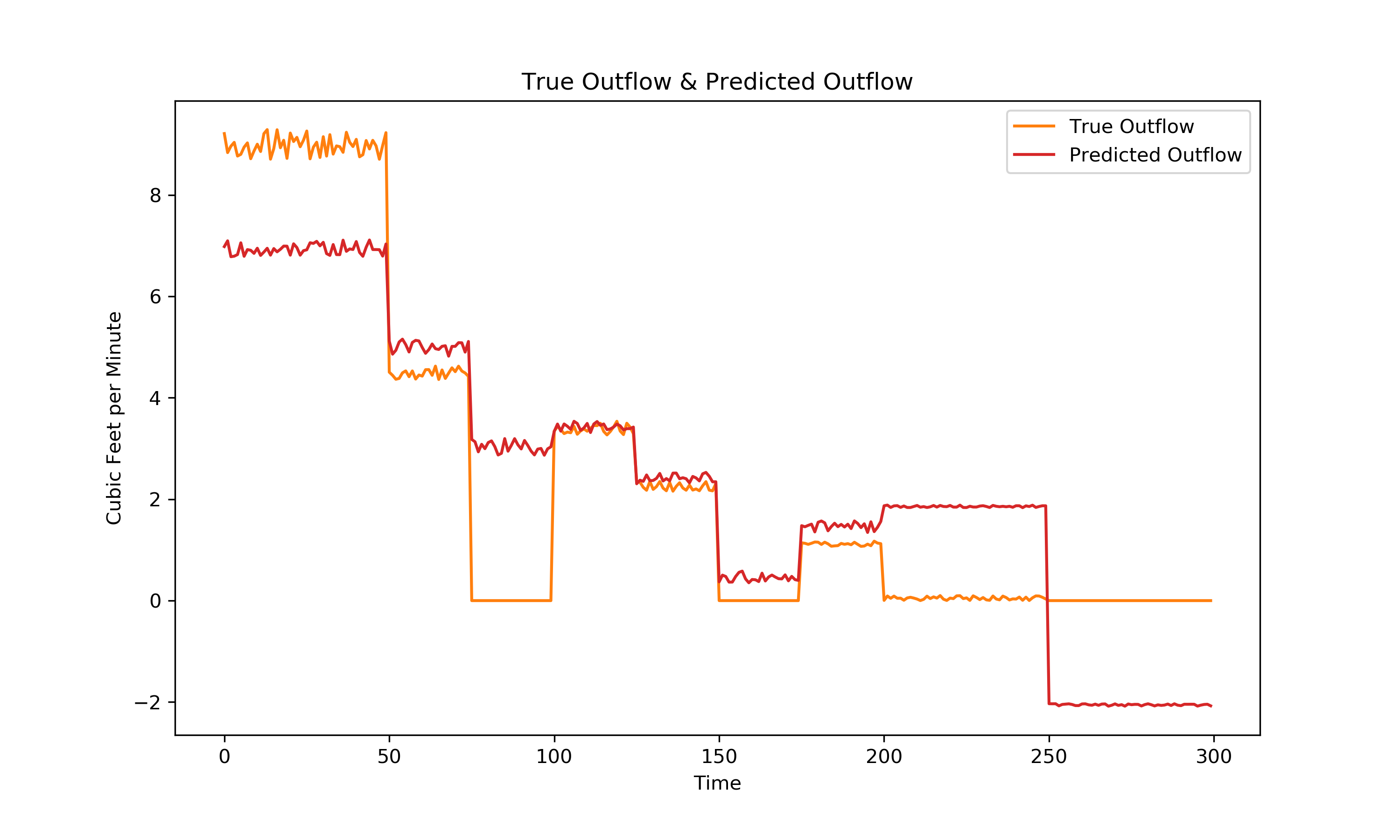
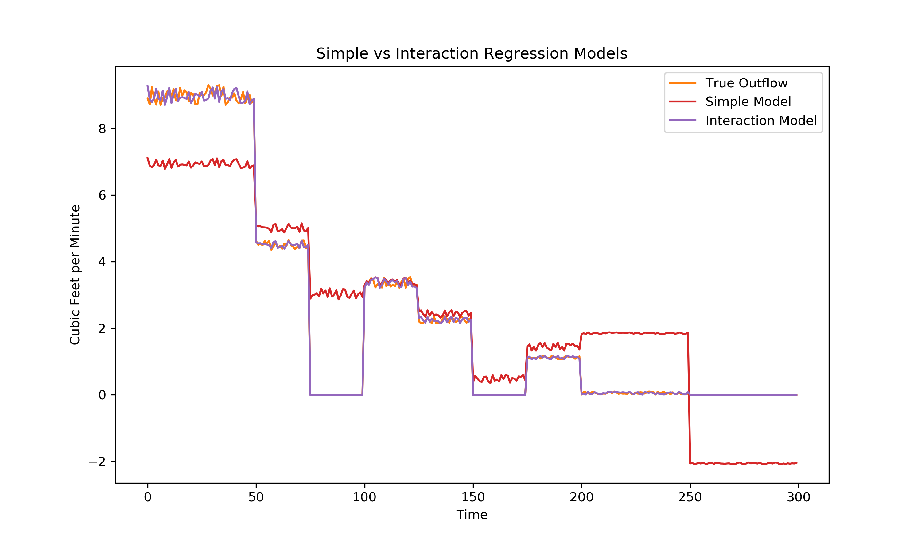
It is clear that the simple linear regression model did not do an excellent job of detecting the relationships in the data. Primarily, I gave no room for the detection of the interaction between valve position and inflow. We can intuit (using the system diagram) that the outflow is a function of the multiplication of inflow and valve position. This is because if the valve is fully open, allowing all air into the outflow, then the outflow is only a function of the inflow and the losses within the ducting. If the valve is fully closed, allowing all air into the exhaust, the outflow is 0. For convenience in this exploration I have set the valve position as values between 0 and 1 with 1 being fully open, though in a real application some additional feature engineering may be required.
The simple linear regression model above had an R² value of .738.
The regression equation:
\(Outflow = \beta _{1}*Inflow + \beta _{2}*Valve Position + \beta _{0}\)
| \(\beta _{0}\) | -2.08 |
| \(\beta _{1}\) | 0.51 |
| \(\beta _{2}\) | 3.91 |
Regression Model with Interaction Term
I’ll add the Inflow * Valve Position interaction term, then regress on the new data set. Excerpt from new data set:
| Inflow | Outflow | ValvePos | Inflow*ValvePos |
| 10.33 | 8.91 | 1 | 10.33 |
| 9.89 | 8.72 | 1 | 9.89 |
| 9.79 | 9.24 | 1 | 9.79 |
| 9.92 | 8.91 | 1 | 9.92 |
| 10.25 | 0 | 0 | 0 |
You might wonder why I don’t just regress on the interaction term directly instead of on inflow, valve position, and inflow * valve position together. According to the hierarchical principal, main effects should be kept in the model, even if the p values associated with their coefficients are not significant. I don’t really understand why fully (or at all), but if you’re interested in exploring more, An Introduction to Statistical Learning has some content on the subject. If you find any good explanation I would be stoked to see it. (I can pay up to 10 dogecoin for your efforts).
Below is the equation (including interaction) as well as the coefficients associated with the independent variables.
\(Outflow = \beta _{1}*Inflow + \beta _{2}*Valve Position + \beta _{3}*Valve Position*Inflow + \beta _{0}\)
| \(\beta _{0}\) | 0 |
| \(\beta _{1}\) | 0 |
| \(\beta _{2}\) | 0 |
| \(\beta _{3}\) | 0.9 |
The reaction term dominated the regression equation at .9. Though interestingly it isn’t 1, which would indicate that maybe there is some loss in the ducting, at the valve, or instrument error. Whatever the case may be, lets plot the regression results:
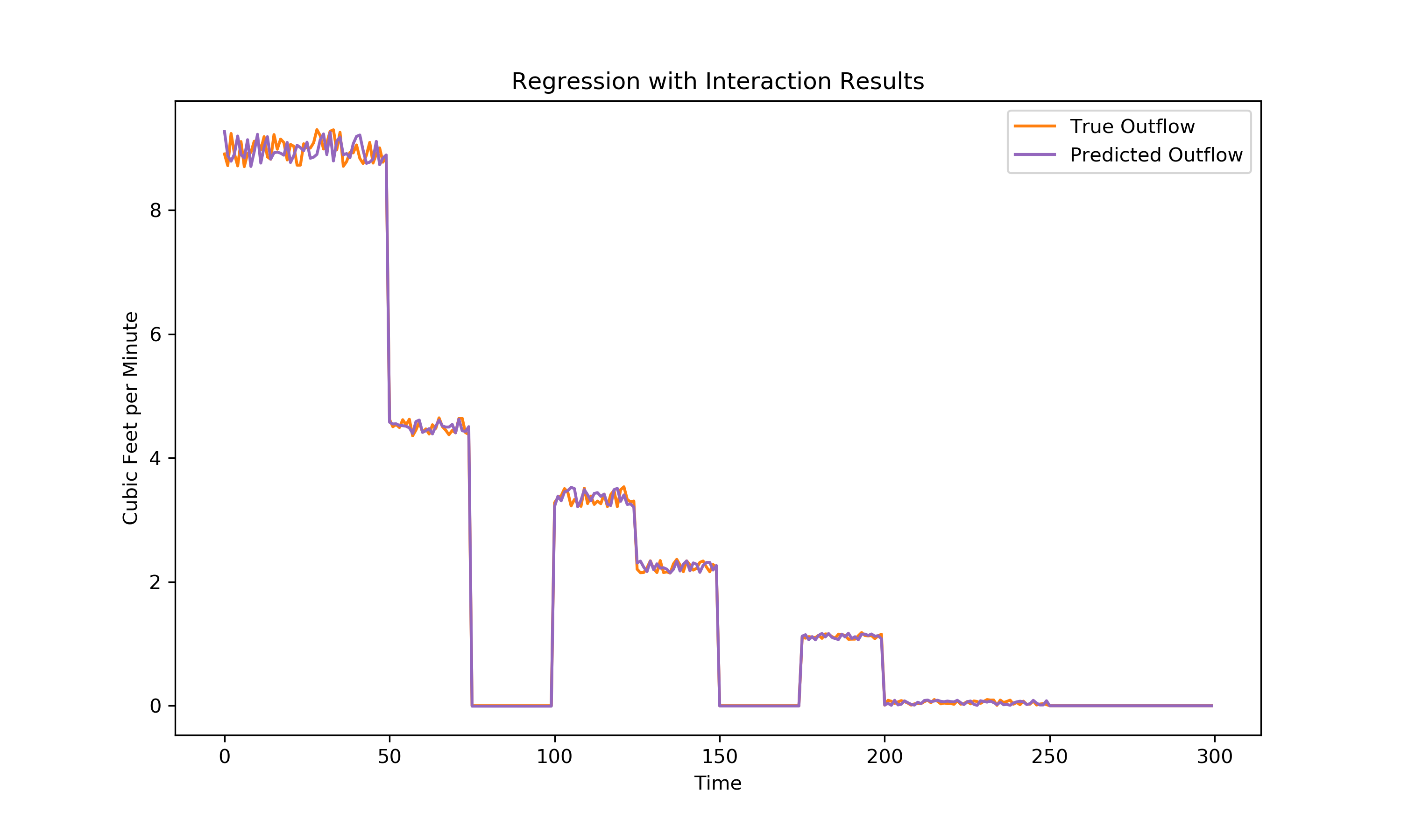
R² value: 0.998
A much better fit than the original model. Lets compare the two models and the true outflow visually:
Closing Thoughts
I am very interested in the ability to detect interaction between terms without domain knowledge about the data set. In the above example, I used knowledge of the system to establish the interaction, but this isn’t always possible or feasible. If you had a very large data set to build models with, it would be interesting to come up with some thoughtful ways to seek out significant interactions. Otherwise, I suppose it could be done in a brute force way, but I would expect there is some risk of overfitting with such a methodology. With enough data, you might be able to avoid over fitting? If you have come across any information on the topic, please share!