On a previous post I suggested it is important to be able to detect interaction in regression analysis in order to create a better model of a dependent variable.
I showed that by creating a new feature (column) in my dataset that represented the known relationship between two other features, a much better multiple linear regression model could be built from the new dataset. In that case, the relationship was multiplicative, but it could be any type of operator or function. The problem with this methodology is that it requires a prior understanding of the relevant interaction between features. It would be slick to be able to detect these feature interactions without prior knowledge.
To recap, given the following three features (plotted over time for better visualization):
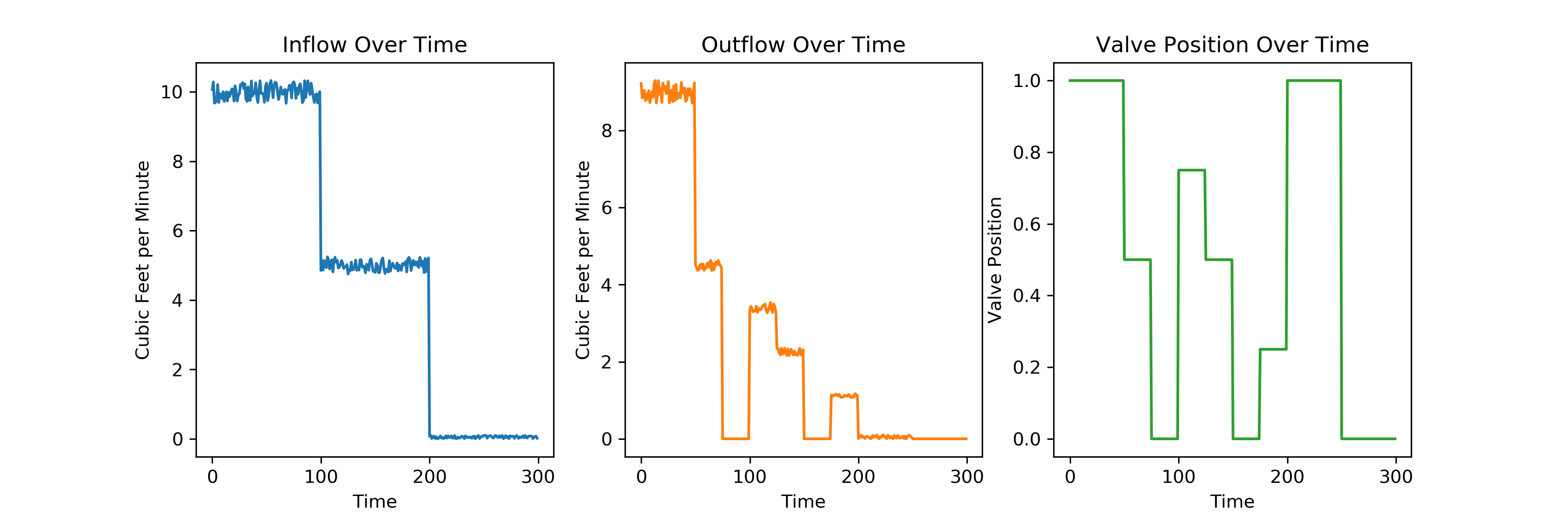
we can create an ordinary least squares regression model that predicts the following on the training set:
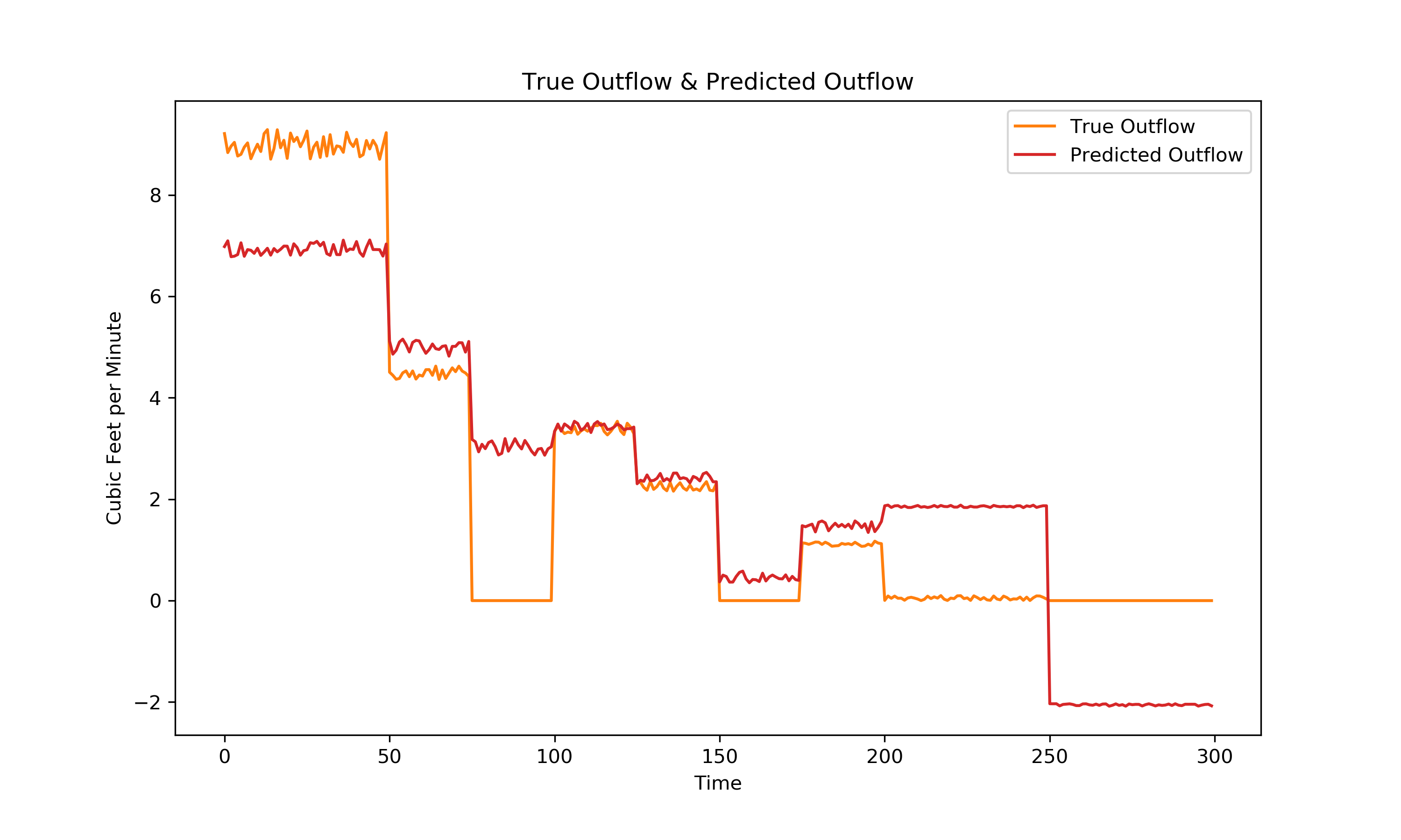
Visually, it is clear this is not a great model. So how can we make a better model without manually finding any non additive relationships? It turns out that it is possible to build a model iteratively that can detect these relationships. The multilayer perceptron model is a type of neural net model that is available through the python’s sci-kit learn package. Fortunately it is highly accessible and is called the MLPRegressor.
Building the Multilayer Perceptron Regression Model
I will have to go over how a multilayer perceptron model is built in a future post. As for now I do not understand it well enough to explain in detail. However, I am excited to learn more about it. Here is a crash course:
Inputs (independent features in the dataset) are passed into layers of hidden units, each unit sums all inputs with some weights and applies a nonlinear activation function to the result which is passed to the next hidden layer. The results eventually pass to the output layer. Weights are updated according to the partial derivates of the loss function. In the case of the default scikit-learn MLPRegressor – the default solver is ‘adam’ which utilizes a modified stochastic gradient descent.
Luckily none of that has to make sense to be able to build an MLPRegressor model successfully.
In the case of this simple dataset (visualized above in the 3 adjacent plots) I built an MLPRegressor with the following commands:
from sklearn.neural_network import MLPRegressor
mlpr = MLPRegressor(max_iter=1000, hidden_layer_sizes=(100,))
mlpr_model = mlpr.fit(df.drop('outflow', axis=1), df['outflow'])
*Note that a jupyter notebook with all python code to walk through this example is available on the Wool Socks GitHub.
Plotting on the training set along with the previously shown multiple ordinary least squares linear regression model:
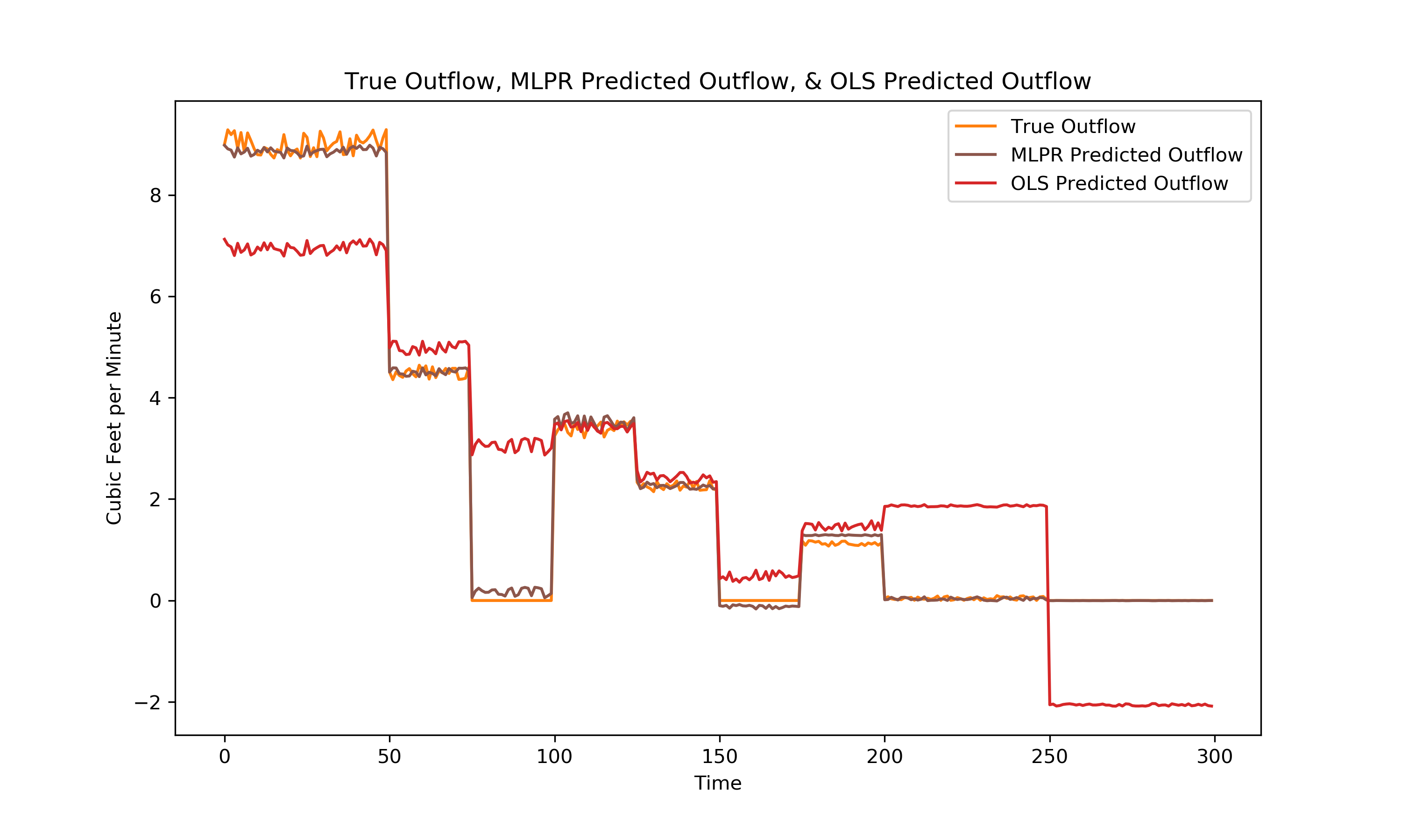
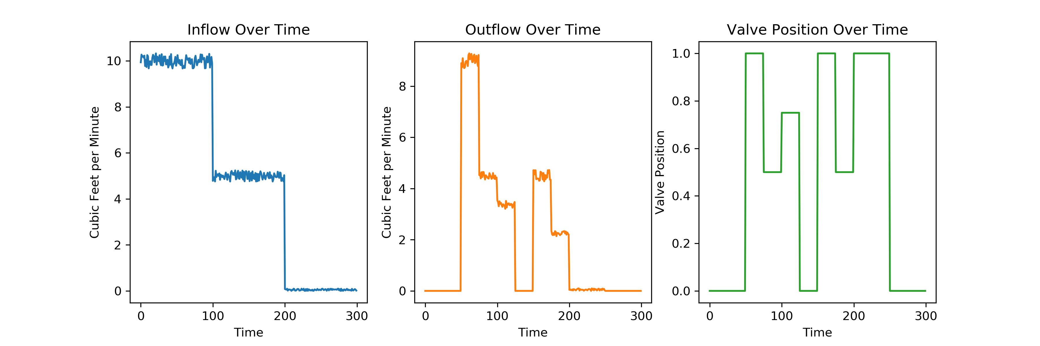
It is clear that the brown MLPR model is a much better predictor on the training data (in comparison to the red OLS model), but as is often the case training set – fit improves with increasing model complexity. The model should be evaluated on a set of test data to properly compare its performance with the ordinary least squares model. Below is a visualization of the test data:
Here are the predicted fits on the test data:

Once again, the multilayer perceptron regression model outperformed the linear regression model. Why? It appears from the result that the MLPR model was able to establish the multiplicative relationship between inflow and valve position without any prior feature engineering. Which is exciting! I am hopeful that this methodology can be useful to detect all kinds of relationships between variables.
Testing Multilayer Perceptron Capability in Detecting Interaction
While I am not yet educated enough on the topic to dive into a detailed analysis on the MLP’s ability to detect all types of interaction, it may be interesting to detect if it is capable of resolving a relationship between variables that is more complex than multiplication. Lets look at a regression model that predicts y in a dataset with additional parameters f(x) and h(x). In python:
x = np.arange(0,300)
fx = np.random.randn(300)
hx = np.random.randn(300)
y = fx**2*np.cos(hx)
f(x) and h(x) are random samples from the standard normal distribution, each of length 300.
y represents the following interaction between the two:
$$ y = f(x)^{2}cos(h(x)) $$
The signals are plotted below:
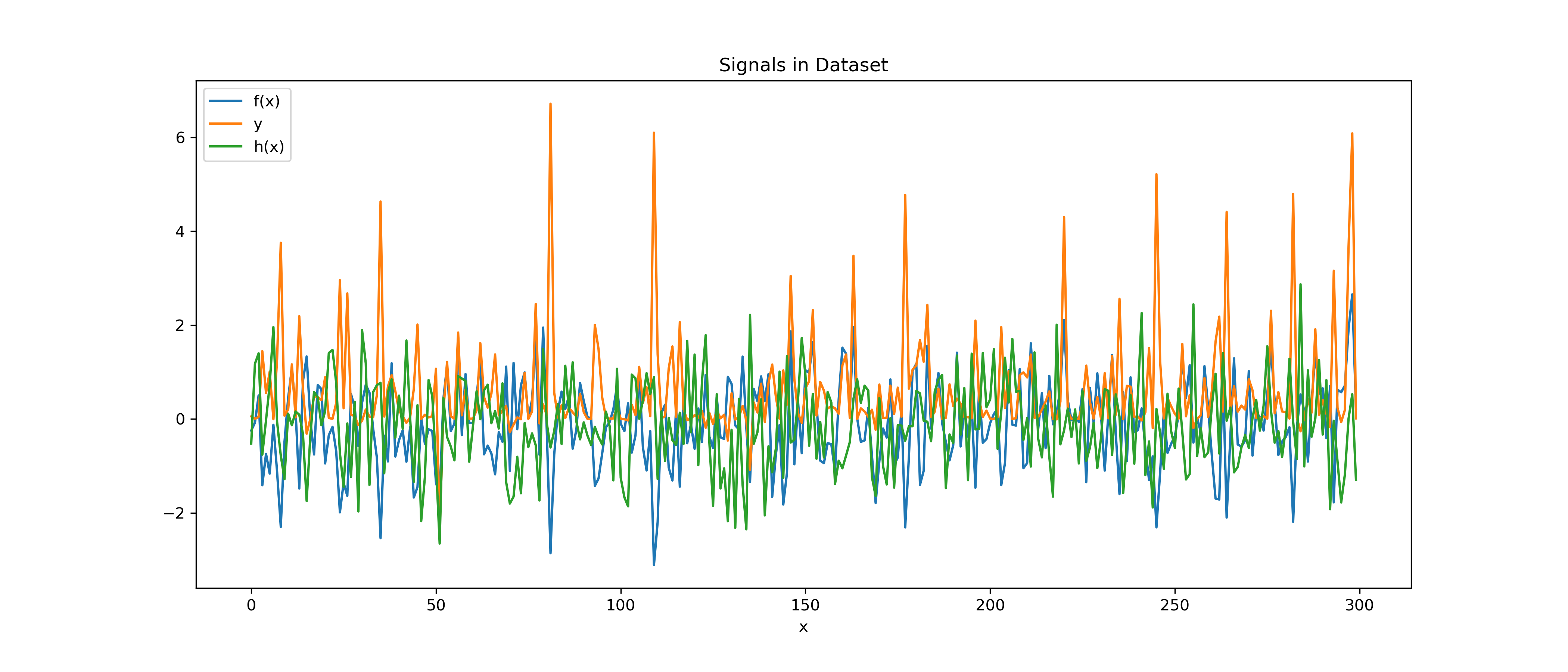
So in this case, we have a dependent variable y that is equal to the square of f(x) multiplied by the cosine of h(x). This seems like a sufficient step up from a simple multiplicative interaction.
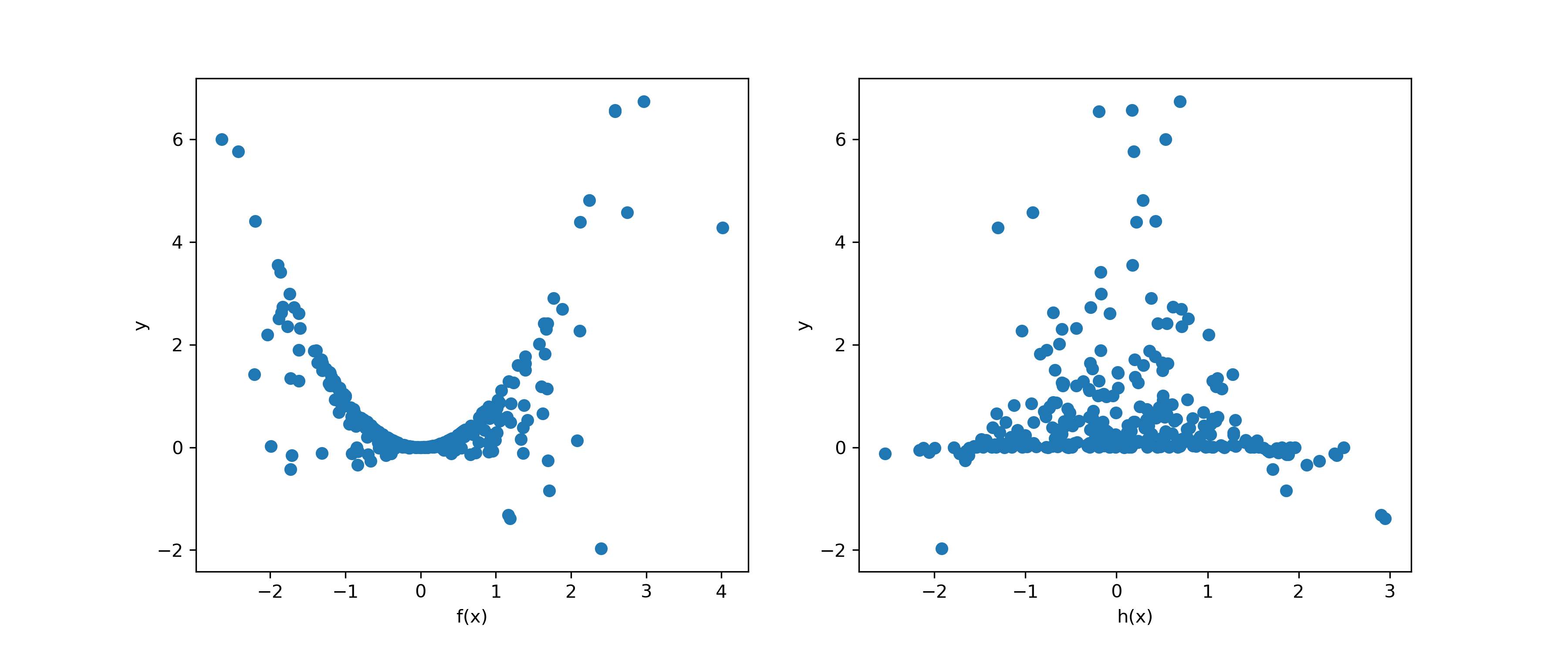
To confirm the lack of linearity between both h(x) and f(x) and y, they are plotted below:
The MLPR model is fitted to the dataset (along with an OLS multiple linear regression model for comparison) with the code below:
mlpr = MLPRegressor(hidden_layer_sizes=(1000,), max_iter=10000, activation = 'relu', solver = 'adam', alpha = .0001)
mlpr_model = mlpr.fit(data_df.drop('g(x)', axis = 1),data_df['g(x)'])
ols_model = lr.fit(data_df.drop('g(x)', axis =1),data_df['g(x)'])
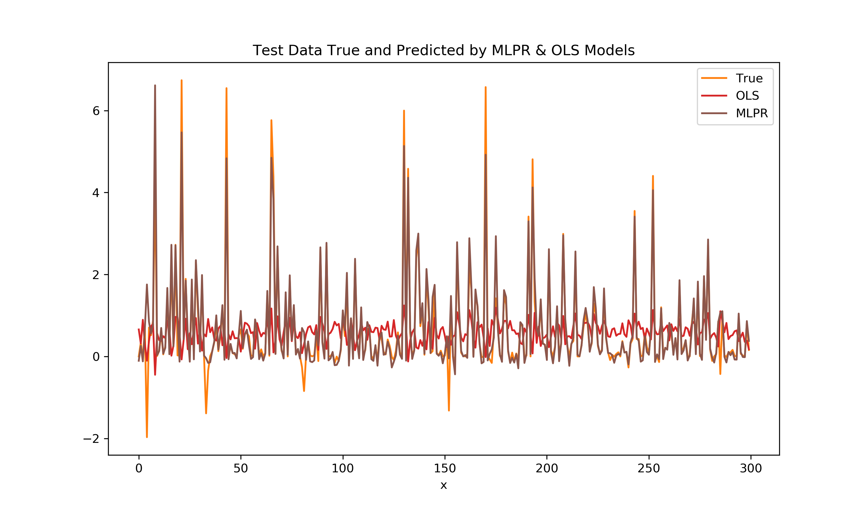
To be sure of the results, a test dataset of another 300 points is made to evaluate the model performance on. The below plot shows the orange test data y signal along with the red OLS predicted signal and the brown MLPR predicted signal.
Since it is difficult to see the different signals, lets look at the error distributions:

A key metric in evaluating the two different fits is the R² Score. In this case the MLPR significantly outperforms the linear model with score differences of:
MLPR R² = 0.96
Linear R² = 0.043
The MLPR model was seemingly able to detect the highly nonlinear relationship between the two variables f(x), h(x), their interaction, and the output y. This was done with no input from the user about the relationships in the data. This could be incredibly useful for developing accurate predictive models on data without having to use prior knowledge or domain knowledge about the dataset to gather insights. Unfortunately, the complexity associated with hundreds of hidden layers, activation functions, and weights results in a significant loss of interpretability.
So in some sense, the title of this post is a misnomer in that I couldn’t tell you the relationship between f(x), h(x), and y from the model. However the model did adequately characterize the relationship for prediction purposes.
An exciting prospect is to apply this type of model to much larger real-world datasets, and more carefully utilize the L2 regularization. Before getting ahead of myself I should understand more about how it works which will be saved for a future post.